Decision Trees

Decision Trees
https://scikit-learn.org/stable/modules/tree.html
Decision Trees (DTs) are a non-parametric supervised learning method used for classification and regression. 

The goal is to create a model that predicts the value of a target variable by learning simple decision rules inferred from the data features. 
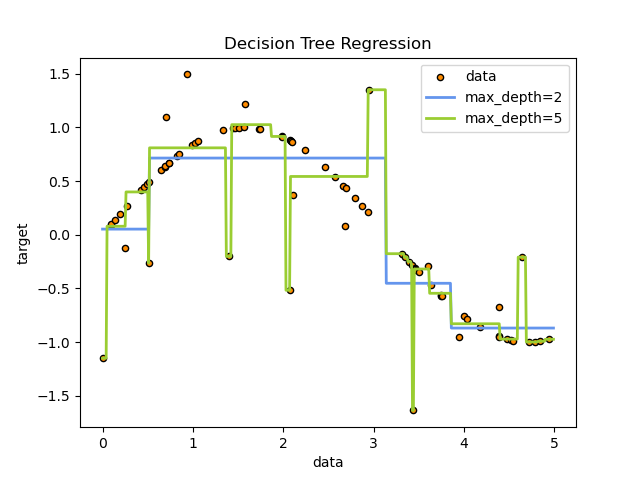
A tree can be seen as a piecewise constant approximation.
For instance, in the example below, decision trees learn from data to approximate a sine curve with a set of if-then-else decision rules. 

The deeper the tree, the more complex the decision rules and the fitter the model.

Some advantages of decision trees are:

Simple to understand and to interpret. 
Trees can be visualized.
Requires little data preparation. 

Other techniques often require data normalization, dummy variables need to be created and blank values to be removed. 
Note however that this module does not support missing values.
The cost of using the tree (i.e., predicting data) is logarithmic in the number of data points used to train the tree.

Able to handle both numerical and categorical data. 
However, the scikit-learn implementation does not support categorical variables for now. 
Other techniques are usually specialized in analyzing datasets that have only one type of variable. 

See algorithms for more information.
Able to handle multi-output problems.
Uses a white box model. 

If a given situation is observable in a model, the explanation for the condition is easily explained by boolean logic.
By contrast, in a black box model (e.g., in an artificial neural network), results may be more difficult to interpret.
Possible to validate a model using statistical tests. 

That makes it possible to account for the reliability of the model.
Performs well even if its assumptions are somewhat violated by the true model from which the data were generated.
The disadvantages of decision trees include:

Decision-tree learners can create over-complex trees that do not generalize the data well. 
This is called overfitting. 
Mechanisms such as pruning, setting the minimum number of samples required at a leaf node or setting the maximum depth of the tree are necessary to avoid this problem.

Decision trees can be unstable because small variations in the data might result in a completely different tree being generated.
This problem is mitigated by using decision trees within an ensemble.
Predictions of decision trees are neither smooth nor continuous, but piecewise constant approximations as seen in the above figure. 

Therefore, they are not good at extrapolation.
The problem of learning an optimal decision tree is known to be NP-complete under several aspects of optimality and even for simple concepts. 
Consequently, practical decision-tree learning algorithms are based on heuristic algorithms such as the greedy algorithm where locally optimal decisions are made at each node. 

Such algorithms cannot guarantee to return the globally optimal decision tree. 
This can be mitigated by training multiple trees in an ensemble learner, where the features and samples are randomly sampled with replacement.
There are concepts that are hard to learn because decision trees do not express them easily, such as XOR, parity or multiplexer problems.

Decision tree learners create biased trees if some classes dominate.
It is therefore recommended to balance the dataset prior to fitting with the decision tree.
1.10.1. Classification
DecisionTreeClassifier is a class capable of performing multi-class classification on a dataset.
As with other classifiers, DecisionTreeClassifier takes as input two arrays:

an array X, sparse or dense, of shape (n_samples, n_features) holding the training samples, and an array Y of integer values, shape (n_samples,), holding the class labels for the training samples:
>>> from sklearn import tree
>>> X = [[0, 0], [1, 1]]

>>> Y = [0, 1]
>>> clf = tree.DecisionTreeClassifier()
>>> clf = clf.fit(X, Y)

After being fitted, the model can then be used to predict the class of samples:
>>> clf.predict([[2., 2.]])
array([1])

In case that there are multiple classes with the same and highest probability, the classifier will predict the class with the lowest index amongst those classes.
As an alternative to outputting a specific class, the probability of each class can be predicted, which is the fraction of training samples of the class in a leaf:
>>> clf.predict_proba([[2., 2.]])

array([[0., 1.]])
DecisionTreeClassifier is capable of both binary (where the labels are [-1, 1]) classification and multiclass (where the labels are [0, …, K-1]) classification.
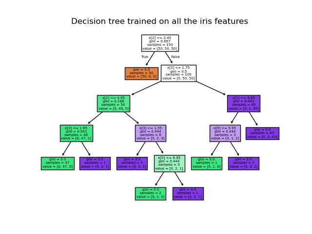
Using the Iris dataset, we can construct a tree as follows:

>>> from sklearn.datasets import load_iris
>>> from sklearn import tree
>>> iris = load_iris()

>>> X, y = iris.data, iris.target
>>> clf = tree.DecisionTreeClassifier()
>>> clf = clf.fit(X, y)

Once trained, you can plot the tree with the plot_tree function:
>>> tree.plot_tree(clf)
[...]


We can also export the tree in Graphviz format using the export_graphviz exporter. 
If you use the conda package manager, the graphviz binaries and the python package can be installed with conda install python-graphviz.

Alternatively binaries for graphviz can be downloaded from the graphviz project homepage, and the Python wrapper installed from pypi with pip install graphviz.
Below is an example graphviz export of the above tree trained on the entire iris dataset; the results are saved in an output file iris.pdf:
>>> import graphviz 

>>> dot_data = tree.export_graphviz(clf, out_file=None) 
>>> graph = graphviz.Source(dot_data) 
>>> graph.render("iris") 

The export_graphviz exporter also supports a variety of aesthetic options, including coloring nodes by their class (or value for regression) and using explicit variable and class names if desired. 
Jupyter notebooks also render these plots inline automatically:
>>> dot_data = tree.export_graphviz(clf, out_file=None, 
... feature_names=iris.feature_names,  
... class_names=iris.target_names,  
... filled=True, rounded=True,  
... special_characters=True)  
>>> graph = graphviz.Source(dot_data)  

>>> graph 



Alternatively, the tree can also be exported in textual format with the function export_text. 
This method doesn’t require the installation of external libraries and is more compact:
>>> from sklearn.datasets import load_iris

>>> from sklearn.tree import DecisionTreeClassifier
>>> from sklearn.tree import export_text
>>> iris = load_iris()

>>> decision_tree = DecisionTreeClassifier(random_state=0, max_depth=2)
>>> decision_tree = decision_tree.fit(iris.data, iris.target)
>>> r = export_text(decision_tree, feature_names=iris['feature_names'])

>>> print(r)
|--- petal width (cm) <= 0.80
|   |--- class: 0
|--- petal width (cm) >  0.80
|   |--- petal width (cm) <= 1.75
|   |   |--- class: 1

|   |--- petal width (cm) >  1.75
|   |   |--- class: 2

Examples:
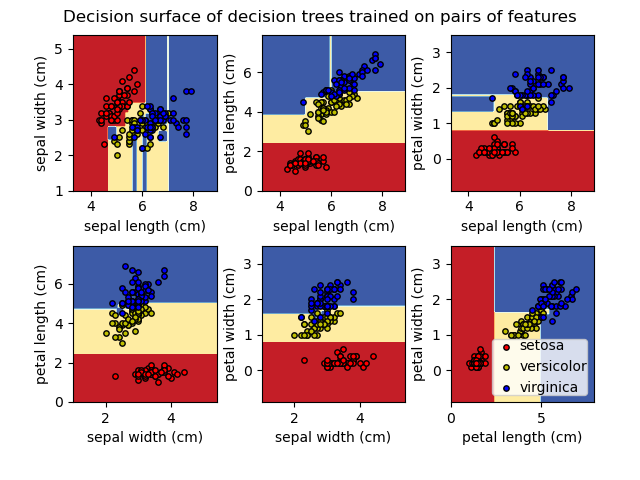
Plot the decision surface of decision trees trained on the iris dataset
Understanding the decision tree structure
1.10.2. 

Regression

Decision trees can also be applied to regression problems, using the

DecisionTreeRegressor class.
As in the classification setting, the fit method will take as argument arrays X and y, only that in this case y is expected to have floating point values instead of integer values:
>>> from sklearn import tree

>>> X = [[0, 0], [2, 2]]
>>> y = [0.5, 2.5]
>>> clf = tree.DecisionTreeRegressor()

>>> clf = clf.fit(X, y)
>>> clf.predict([[1, 1]])
array([0.5])

Examples:
Decision Tree Regression
1.10.3. 

Multi-output problems
A multi-output problem is a supervised learning problem with several outputs to predict, that is when Y is a 2d array of shape (n_samples, n_outputs).
When there is no correlation between the outputs, a very simple way to solve this kind of problem is to build n independent models, i.e. 

one for each output, and then to use those models to independently predict each one of the n outputs. 
However, because it is likely that the output values related to the same input are themselves correlated, an often better way is to build a single model capable of predicting simultaneously all n outputs. 
First, it requires lower training time since only a single estimator is built. 

Second, the generalization accuracy of the resulting estimator may often be increased.
With regard to decision trees, this strategy can readily be used to support multi-output problems. 
This requires the following changes:

Store n output values in leaves, instead of 1;
Use splitting criteria that compute the average reduction across all n outputs.
This module offers support for multi-output problems by implementing this strategy in both DecisionTreeClassifier and

DecisionTreeRegressor. 
If a decision tree is fit on an output array Y of shape (n_samples, n_outputs) then the resulting estimator will:
Output n_output values upon predict;

Output a list of n_output arrays of class probabilities upon
predict_proba.
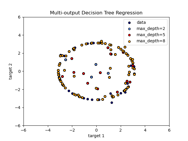
The use of multi-output trees for regression is demonstrated in

Multi-output Decision Tree Regression. 
In this example, the input
X is a single real value and the outputs Y are the sine and cosine of X.


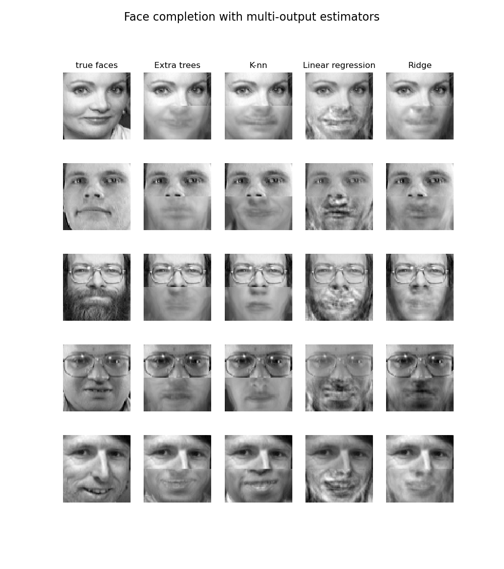
The use of multi-output trees for classification is demonstrated in
Face completion with a multi-output estimators. 

In this example, the inputs
X are the pixels of the upper half of faces and the outputs Y are the pixels of the lower half of those faces.


Examples:
Multi-output Decision Tree Regression
Face completion with a multi-output estimators

Random Forest
As is implied by the names "Tree" and "Forest," a Random Forest is essentially a collection of Decision Trees. 
A decision tree is built on an entire dataset, using all the features/variables of interest, whereas a random forest randomly selects observations/rows and specific features/variables to build multiple decision trees from and then averages the results. 

After a large number of trees are built using this method, each tree "votes" or chooses the class, and the class receiving the most votes by a simple majority is the "winner" or predicted class. 
There are of course some more detailed differences, but this is the main conceptual difference.